pip install attention pip install keras_tuner import os import re import itertools import numpy as np import scipy.signal import pandas as pd import seaborn as sns import scipy.io as scio import tensorflow as tf import keras_tuner as kt import matplotlib.pyplot as plt   from sklearn.svm import SVC from sklearn import preprocessing from sklearn.utils import shuffle from sklearn.neural_network import MLPClassifier from sklearn.neighbors import KNeighborsClassifier from sklearn.ensemble import RandomForestClassifier from sklearn.model_selection import train_test_split from sklearn.preprocessing import LabelBinarizer, OneHotEncoder, StandardScaler from sklearn.metrics import confusion_matrix, ConfusionMatrixDisplay, classification_report, confusion_matrix, precision_score, recall_score, f1_score, accuracy_score, roc_curve, roc_auc_score, auc   from tensorflow import keras   from keras.layers import * from keras import backend as k from keras.optimizers import Adam from keras.models import Sequential,Model,load_model from keras.callbacks import ReduceLROnPlateau, ModelCheckpoint   from tensorflow.keras.models import Sequential,Model from tensorflow.keras.layers import Input,Dense, Dropout, Flatten, Conv1D, MaxPooling1D   from attention import Attention from google.colab import drive drive.mount('/content/drive')

Data Visualization

working_cond = 40 #this corresponds to possible values under which the voltage source operates i.e., 40, 80 and 120   Path = r'/content/drive/MyDrive/ALL_DC_motor_Data/Ua_120V_Noise_2_perct'.format(working_cond) # Path of the folder containing CSV files from that working condition file_name = os.listdir(path=Path) # List of all the files in the folder fig, axs = plt.subplots(len(file_name), 2, figsize=(10, 2 * len(file_name)))   for i, file in enumerate(file_name):     csv_path = os.path.join(Path, file) # Obtains the exact path for that file     df = pd.read_csv(csv_path)  # saves that Fault data in a dummy variable "df"     df = df.iloc[::50]     ax1 = axs[i][0]     ax2 = axs[i][1]     ax1.plot(df['time'], df['a1_lower'], '-r', label='')     ax2.plot(df['time'], df['a2_lower'], '-r', label='')     ax1.plot(df['time'], df['a1_upper'], '-g', label='a1')     ax2.plot(df['time'], df['a2_upper'], '-g', label='a2')     ax1.plot(df['time'], df['ARR1'], '-b', label='')     ax2.plot(df['time'], df['ARR2'], '-b', label='')     ax1.set_title(file[:-13]) #to extract only the fault type from the name of fault file, _noise_02.csv contains 13 characters     ax1.set_ylim(-30, 30)     ax1.set_xlabel('Time')     ax1.set_ylabel('r1')     ax2.set_title(file[:-13])     ax2.set_ylim(-1, 1)     ax2.set_xlabel('Time')     ax2.set_ylabel('r2')   plt.tight_layout() plt.show()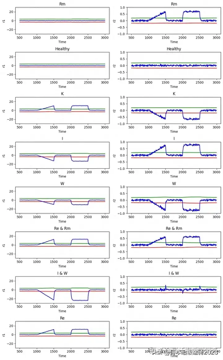

Path = r'/content/drive/MyDrive/ALL_DC_motor_Data/Ua_120V_Noise_2_perct'.format(40) # Path of the folder containing CSV files from that working condition file_name = os.listdir(path=Path) # List of all the files in the folder   fig, axs = plt.subplots(len(file_name), 2, figsize=(10, 2 * len(file_name)))   for i, file in enumerate(file_name):     csv_path = os.path.join(Path, file)     df = pd.read_csv(csv_path)     df = df.iloc[::50]     ax1 = axs[i][0]     ax2 = axs[i][1]     ax1.plot(df['time'], df['Im'], '-r', label='')     ax2.plot(df['time'], df['Wm'], '-b', label='')     ax1.set_title(file[:-13])     ax1.set_ylim(20, 36)     ax1.set_xlabel('Time')     ax1.set_ylabel('$I_m$')     ax2.set_title(file[:-13])     ax2.set_ylim(250, 480)     ax2.set_xlabel('Time')     ax2.set_ylabel('$\omega_m$')   plt.tight_layout() plt.show()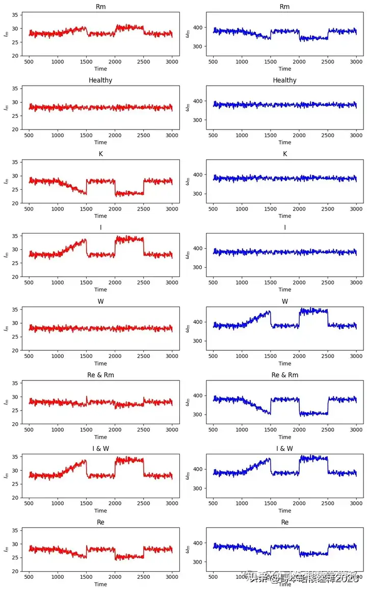

Dataframe Creation

def obtain_DataFrame_for_this_working_condition(working_cond):     # Input = "Working Condition" [40V, 80V, 120V]     # Output = "A dataFrame contaning all fault scnerio from that Working Condition"     # The DataFrame has following columns [time, I, W, ARR1, ARR2, a1_upper,  a1_lower, a2_upper,  a2_lower,  activation_arr1,  activation_arr2 FaultClass] for the given "working_cond"       Path = r'/content/drive/MyDrive/ALL_DC_motor_Data/Ua_{}V_Noise_2_perct'.format(working_cond) # Path of the folder containing CSV files from that working condition     file_name = os.listdir(path=Path) # List of all the files in the folder       DF = pd.DataFrame() # Initialize an empty DataFrame       for f in file_name : #Iterate through each file, which coresponds to a Fault           csv_path =  os.path.join(Path,f) #Obtains the exact path for that file           df = pd.read_csv(csv_path) #saves that Fault data in a dummy variable "df"             temp1=df[(df.time > 1050) & (df.time< 1500)]  # Incipient Faults -----Taking samples after which the fault was introduced           temp2=df[(df.time > 2050) & (df.time< 2500)]  # Step Faults-----------Taking samples after which the fault was introduced           df=pd.concat([temp1,temp2])                  #Concatinate both Incipient and Step Fault           DF=pd.concat([DF,df])                        # Append the "f"-Fault to the new dataframe DF       DF['Working_cond'] = np.repeat('U-{}V'.format(working_cond), len(DF))     return DF df_120 = obtain_DataFrame_for_this_working_condition(working_cond=120) df_40 = obtain_DataFrame_for_this_working_condition(working_cond=40) df_80 = obtain_DataFrame_for_this_working_condition(working_cond=80)   DF = pd.concat([df_40,df_80,df_120]) # ALL 3 working conditions are saved in one DataFRame sns.scatterplot(data=DF.iloc[::400,:],x='Im',y='Wm',hue='Fault_type',style='Fault_type',edgecolor='black') plt.legend() plt.show()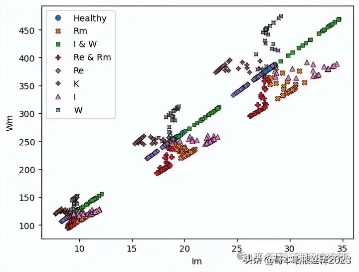

sns.scatterplot(data=DF.iloc[::200,:],x='ARR1',y='ARR2',style='Fault_type',hue='Fault_type', palette = 'deep', edgecolor = 'black') plt.legend() plt.show()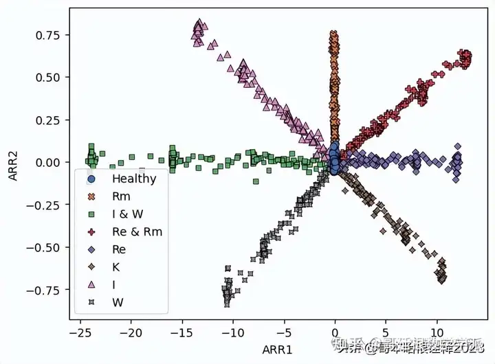

Data Augmentation

def Sliding_Window(df_temp, win_len, stride):     """     Sliding window function for data segmentation and label extraction.       Args:         df_temp (DataFrame): Input dataframe containing the data.         win_len (int): Length of the sliding window.         stride (int): Stride or step size for sliding the window.       Returns:         X (ndarray): Segmented input sequences.         Y (ndarray): Extracted output labels.         T (ndarray): Corresponding timestamps.     """     X = []  # List to store segmented input sequences.     Y = []  # List to store extracted output labels.     T = []  # List to store corresponding timestamps.       # Loop through the dataframe with the specified stride.     for i in np.arange(0, len(df_temp) - win_len, stride):         # Extract a subset of the dataframe based on the window length.         temp = df_temp.iloc[i:i + win_len, [3, 4]].values           # Append the segmented input sequence to the X list.         X.append(temp)           # Append the output label at the end of the window to the Y list.         Y.append(df_temp.iloc[i + win_len, -1])           # Append the timestamp at the end of the window to the T list.         T.append(df_temp.iloc[i + win_len, 0])       return np.array(X), np.array(Y), np.array(T)

Data Preprocessing

def PreprocessData(working_cond, win_len, stride):     """     Preprocessing function to extract input sequences and output labels from CSV files of a specific working condition.       Args:         working_cond (str): Working condition identifier used to locate the folder containing CSV files.         win_len (int): Length of the sliding window.         stride (int): Stride or step size for sliding the window.       Returns:         X_full (ndarray): Concatenated segmented input sequences.         Y_full (ndarray): Concatenated output labels.     """       Path = r'/content/drive/MyDrive/ALL_DC_motor_Data/Ua_{}V_Noise_2_perct'.format(working_cond)     file_name = os.listdir(path=Path)       X_full, Y_full = [], []  # Lists to store concatenated segmented input sequences and output labels       for f in file_name:  # Iterate through each file, which corresponds to a fault         csv_path = os.path.join(Path, f)         df = pd.read_csv(csv_path)           temp_df_1 = df[(df.time > 1050) & (df.time < 1500)]  # Incipient - Taking samples after which the parameter fault was introduced         x1, y1, _ = Sliding_Window(temp_df_1, win_len, stride)           temp_df_2 = df[(df.time > 2050) & (df.time < 2500)]  # Step - Taking samples after which the parameter fault was introduced         x2, y2, _ = Sliding_Window(temp_df_2, win_len, stride)           x_temp, y_temp = np.concatenate((x1, x2), axis=0), np.concatenate((y1, y2), axis=0)           X_full.append(x_temp)         Y_full.append(y_temp)       X_full = np.array(X_full)     X_full = np.reshape(X_full, (-1, X_full.shape[2], X_full.shape[3]))       Y_full = np.array(Y_full)     Y_full = np.reshape(Y_full, (-1))       return X_full, Y_full WL=20 # can be used for adjusting window length S=40 # can be used for adjusting stride   # Preprocess data for working condition 120 X_120, Y_120 = PreprocessData(working_cond=120, win_len=WL, stride=S)   # Preprocess data for working condition 80 X_80, Y_80 = PreprocessData(working_cond=80, win_len=WL, stride=S)   # Preprocess data for working condition 40 X_40, Y_40 = PreprocessData(working_cond=40, win_len=WL, stride=S)   # Concatenate the preprocessed data from different working conditions X_full = np.concatenate((X_40, X_80, X_120)) Y_full = np.concatenate((Y_40, Y_80, Y_120)) # Train Test split X_train, X_test, y_train, y_test = train_test_split(X_full, Y_full, train_size=256, random_state=42)   # Standardising the data scaler = StandardScaler() X_train_sc = scaler.fit_transform(X_train.reshape(-1,X_train.shape[-1])).reshape(X_train.shape) X_test_sc = scaler.transform(X_test.reshape(-1,X_test.shape[-1])).reshape(X_test.shape)   # One Hot encoding encoder = OneHotEncoder(sparse_output=False) # in case of error, add the argument handle_unknown = 'ignore'   y_train_ohe = encoder.fit_transform(y_train.reshape(-1,1)) y_test_ohe = encoder.transform(y_test.reshape(-1,1))

Model Architecture

def build_model(hp):       num_classes=len(encoder.categories_[0])       # create model object     model = Sequential([     Conv1D(filters=hp.Int('conv_1_filter', min_value=16, max_value=128, step=32), kernel_size=hp.Choice('conv_1_kernel', values = [3,5]), activation='relu', input_shape=(X_train.shape[1],X_train.shape[2]), padding='same'),     MaxPooling1D(pool_size=2,padding='same'),     LSTM(units=hp.Int('lstm_1', min_value=16, max_value=128, step=32), return_sequences=True),     Dropout(0.2),     LSTM(units=hp.Int('lstm_2', min_value=16, max_value=128, step=32), return_sequences=True),     LSTM(units=hp.Int('lstm_3', min_value=16, max_value=128, step=32), return_sequences=True),     Dropout(0.5),     Attention(),     Dense(units=hp.Int('dense_1_units', min_value=32, max_value=128, step=16), activation='relu'),     Dense(num_classes, activation='softmax')     ])       model.compile(optimizer=keras.optimizers.Adam(hp.Choice('learning_rate', values=[1e-2, 1e-3])), loss='categorical_crossentropy', metrics=['accuracy'])       return model tuner = kt.RandomSearch(build_model, objective='val_accuracy', max_trials = 10) #creating randomsearch object tuner.search(X_train_sc,y_train_ohe,epochs=20,validation_data=(X_test_sc,y_test_ohe)) # search best parameter values HyDeLA_model_tuned=tuner.get_best_models(num_models=1)[0] HyDeLA_model_tuned.summary() def HYDELA_model(encoder,X_train_transformed):     num_classes=len(encoder.categories_[0])       HyDeLA_model = Sequential()     HyDeLA_model.add(Conv1D(16, kernel_size=(5),activation='relu',input_shape=(X_train_transformed.shape[1],X_train_transformed.shape[2]),padding='same'))     HyDeLA_model.add(MaxPooling1D((2),padding='same'))     HyDeLA_model.add(LSTM(112, return_sequences=True))     HyDeLA_model.add(Dropout(0.2))     HyDeLA_model.add(LSTM(16,return_sequences=True))     HyDeLA_model.add(LSTM(48,return_sequences=True))     HyDeLA_model.add(Dropout(0.5))     HyDeLA_model.add(Attention())     HyDeLA_model.add(Flatten())     HyDeLA_model.add(Dense(64, activation='relu'))     HyDeLA_model.add(Dense(num_classes, activation='softmax'))       HyDeLA_model.compile(loss='categorical_crossentropy', optimizer=Adam(learning_rate=0.001),metrics=['accuracy'])       return HyDeLA_model

Model Training

# Define an EarlyStopping callback to monitor validation accuracy and restore best weights callback = tf.keras.callbacks.EarlyStopping(monitor='val_accuracy', patience=10, restore_best_weights=True)   # Create a model using the specified encoder and X_train_sc hydela_model = HYDELA_model(encoder, X_train_sc)   # Train the model history = hydela_model.fit(X_train_sc, y_train_ohe, epochs=200, batch_size=16, validation_data=(X_test_sc, y_test_ohe), callbacks=[callback], shuffle=False, verbose=1) # Access the loss values training_loss = history.history['loss'] validation_loss = history.history['val_loss']   epochs = range(1, len(training_loss) + 1)   plt.plot(epochs, training_loss, label='Training loss', marker = 'o', lw = 1) plt.plot(epochs, validation_loss, label='Validation loss', marker = 'x', lw = 1) plt.xlabel('Number of Epochs') plt.ylabel('Loss') plt.title('Training and Validation Loss vs Number of Epochs') plt.legend() plt.show()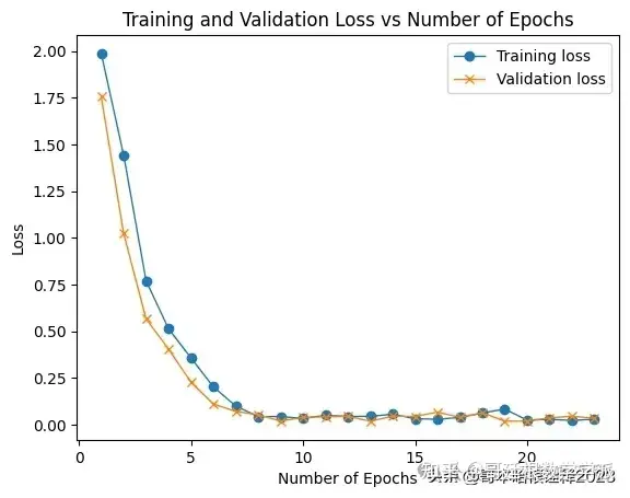

Model Evaluation

# Perform prediction using the CNN model on the scaled test data y_pred = hydela_model.predict(X_test_sc)   # Inverse transform the predicted labels using the encoder y_pred = encoder.inverse_transform(y_pred)   # Calculate and print precision, recall, F1-score and accuracy precision = precision_score(y_test, y_pred, average='weighted') recall = recall_score(y_test, y_pred, average='weighted') f1 = f1_score(y_test, y_pred, average='weighted') accuracy = accuracy_score(y_test, y_pred)   print(f"Training Sample Size = {len(X_train)}, F1 score is - {f1}") print(f"Training Sample Size = {len(X_train)}, Accuracy is - {accuracy}") print(f"Training Sample Size = {len(X_train)}, Precision is - {precision}") print(f"Training Sample Size = {len(X_train)}, Recall is - {recall}") 160/160 [==============================] - 3s 8ms/step Training Sample Size = 256, F1 score is - 0.9947349330945912 Training Sample Size = 256, Accuracy is - 0.9947265625 Training Sample Size = 256, Precision is - 0.9947711101749215 Training Sample Size = 256, Recall is - 0.9947265625 # Define the class labels class_labels = ['Healthy', 'Re', 'Rm', 'I', 'W', 'K', 'Re & Rm', 'I & W']   # Create the confusion matrix conf_matrix = confusion_matrix(y_test, y_pred)   # Create a heatmap plt.figure(figsize=(8, 6)) sns.heatmap(conf_matrix, annot=True, cmap='Reds', fmt='d', xticklabels=class_labels, yticklabels=class_labels) plt.xlabel("Predicted Labels") plt.ylabel("Actual Labels") plt.title("Confusion Matrix") plt.show()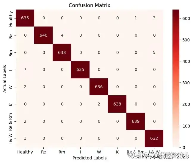

def lab_to_num(value):   """   lab_to_num converts the literal labels to numeric labels as per the mapping function label_mapping = {'Re': 1, 'Rm': 2, 'I': 3, 'W': 4, 'K': 5, 'I & W': 7, 'Re & Rm': 6}   parameter : value is assumed to be numpy.ndarray()   """   for i in range(len(value)):     if value[i]=='Re':       value[i]=1     elif value[i]=='Rm':       value[i]=2     elif value[i]=='I':       value[i]=3     elif value[i]=='W':       value[i]=4     elif value[i]=='K':       value[i]=5     elif value[i]=='I & W':       value[i]=7     elif value[i]=='Re & Rm':       value[i]=6     else:       value[i]=0     return value num_label = ['1', '2', '3', '4', '5', '6', '7']   test_roc = [] pred_roc = []   test_roc = [1 if label in num_label else 0 for label in lab_to_num(y_test)] pred_roc = [1 if label in num_label else 0 for label in lab_to_num(y_pred)] # Compute ROC curve fpr, tpr, threshold = roc_curve(test_roc, pred_roc)   # Compute AUC (Area Under the Curve) roc_auc = auc(fpr, tpr)   # Plot ROC curve plt.figure(figsize=(8, 6)) plt.plot(fpr, tpr, color='b', lw=2, label=f"AUC = {roc_auc:.2f}") plt.plot([0, 1], [0, 1], color='gray', linestyle='--') plt.xlim([-0.05, 1.05]) plt.ylim([-0.05, 1.05]) plt.xlabel('False Positive Rate (FPR)') plt.ylabel('True Positive Rate (TPR)') plt.title('Receiver Operating Characteristic (ROC) Curve') plt.legend(loc="lower right") plt.show()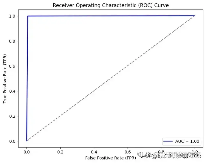

  擅长领域：现代信号处理，机器学习，深度学习，数字孪生，时间序列分析，设备缺陷检测、设备异常检测、设备智能故障诊断与健康管理PHM等。 知乎学术咨询：https://www.zhihu.com/consult/people/792359672131756032?isMe=1 擅长领域：现代信号处理，机器学习，深度学习，数字孪生，时间序列分析，设备缺陷检测、设备异常检测、设备智能故障诊断与健康管理PHM等。

擅长领域：现代信号处理，机器学习，深度学习，数字孪生，时间序列分析，设备缺陷检测、设备异常检测、设备智能故障诊断与健康管理PHM等。