希尔伯特变换

1 特征描述

希尔伯特变换广泛使用于信号处理应用中，以获得信号的解析表示。其可以计算瞬时频率和相位，相位被定义为原始信号和信号的希尔伯特变换之间的角度。对于信号 x ( t ) x(t) x(t)，其希尔伯特变换定义如下。

x ^ ( t ) = H [ x ( t ) ] = 1 π ∫ − ∞ + ∞ x ( τ ) t − τ   d τ \hat{x}(t)=H[x(t)]=\frac{1}{\pi}\int_{-\infty}^{+\infty}\frac{x(\tau)}{t-\tau}\,\text{d}\tau x^(t)=H[x(t)]=π1​∫−∞+∞​t−τx(τ)​dτ

由上式可知，随着变换的结果，自变量不变，因此输出 x ^ ( t ) \hat{x}(t) x^(t)也是与时间有关的函数。此外， x ^ ( t ) \hat{x}(t) x^(t)是 x ( t ) x(t) x(t)的线性函数。它是由 ( π t ) − 1 {({\pi}t)}^{-1} (πt)−1与 x ( t ) x(t) x(t)卷积获得的，如下关系所示。

x ^ ( t ) = 1 π t   ∗   x ( t ) \hat{x}(t)=\frac{1}{{\pi}t}\,\ast\,x(t) x^(t)=πt1​∗x(t)

由上式可以得到 x ( t ) x(t) x(t)的希尔伯特变换的傅立叶变换如下所示。

F [ x ^ ( t ) ] = F [ 1 π t ] F [ x ( t ) ] = − j   s g n ( f ) F [ x ( t ) ] \begin{split} F[\hat{x}(t)]&=F[\frac{1}{{\pi}t}]F[x(t)] \\ &=-j\,sgn(f)F[x(t)] \end{split} F[x^(t)]​=F[πt1​]F[x(t)]=−jsgn(f)F[x(t)]​

其中， s g n ( f ) sgn(f) sgn(f)如下所示。

s g n ( f ) = { + 1 , f > 0 0 , f = 0 − 1 , f < 0 sgn(f)= \begin{cases} \begin{split} +1,&{\quad}f>0\\ 0,&{\quad}f=0\\ -1,&{\quad}f<0 \end{split} \end{cases} sgn(f)=⎩⎨⎧​+1,0,−1,​f>0f=0f<0​​

希尔伯特变换对实际数据作90度相移，正弦变为余弦，反之亦然。希尔伯特变换可用于从实际信号中产生解析信号，解析信号在通信领域中很有用，尤其是在带通信号处理中。解析信号如下所示。

s ( t ) = x ( t ) + j x ^ ( t ) s(t)=x(t)+j\hat{x}(t) s(t)=x(t)+jx^(t)

解析信号的实部是原始的信号数据，虚部是实际的希尔伯特变换结果。

2 数据来源

提供一串信号的数据:
这组数据存在三个频率分量，分别为100Hz，200Hz和300Hz, 用MATLAB生成。

# 定义三个频率分量的参数 t = 0:0.0001:2/100;  freq1 = 100; # 第一个频率分量的频率(Hz) freq2 = 200; # 第二个频率分量的频率(Hz) freq3 = 300; # 第三个频率分量的频率(Hz)  # 生成三个频率分量的正弦波信号 signal1 = sin(2 * pi * freq1 * t); signal2 = sin(2 * pi * freq2 * t); signal3 = sin(2 * pi * freq3 * t);  # 将三个频率分量的信号相加 result = signal1 + signal2 + signal3; 

3 函数的Python代码

3.1 Python库要求

from scipy import signal 

3.2 hilbert希尔伯特变换函数

其中，inputS为输入的信号序列，函数的返回值outputS为解析信号序列。解析信号的实部是原始的信号数据，虚部是实际的希尔伯特变换结果。

outputS = signal.hilbert(inputS) 

3.3 希尔伯特变换函数hilbert验证

from scipy import signal  inputS = input().split()  outputS = signal.hilbert(inputS)  for i in outputS:     print("{} ".format(i.imag), end='') 

4 函数的C++代码

4.1 C++库要求

#include #include #include #include 

4.2 void HilbertTransform(vector &cinS, vector> &outputS)希尔伯特变换函数

其中，cinS为输入的信号序列，outputS为得到的解析信号序列。解析信号的实部是原始的信号数据，虚部是实际的希尔伯特变换结果。

void HilbertTransform(vector &cinS, vector> &outputS) {      //flag=-1时为正变换, flag=1时为反变换     auto dft = [](vector> &Data, int flag) {          int length = Data.size();         complex wn;         vector> temp(length);                  for (size_t i = 0; i < length; i++) {             temp[i] = 0.;             for (size_t j = 0; j < length; j++) {                 wn = complex(cos(2. * acos(-1) / length * i * j), sin(flag * 2. * acos(-1) / length * i * j));                 temp[i] = temp[i] + Data[j] * wn;             }         }          if (flag == -1) {             Data = temp;         } else if (flag == 1) {             for (size_t i = 0; i < length; i++) {                 Data[i] = temp[i] / double(length);             }         }         return;     };     int length = cinS.size();     outputS.resize(length);      for (size_t i = 0; i < length; i++) {         outputS[i].real(cinS[i]);         outputS[i].imag(0.);     }     dft(outputS, -1); //DFT     int half = ((length % 2) == 0) ? (length / 2) : ((length + 1) / 2);     for (size_t i = half; i < length; i++) {         outputS[i] = 0.;     }     dft(outputS, 1); //IDFT     for (size_t i = 0; i < length; i++) {         outputS[i] = 2. * outputS[i];     }     return; } 

4.3 希尔伯特变换函数void HilbertTransform(vector &cinS, vector> &outputS)验证

int main() {      double temp;     vector cinS;     vector> outputS;      int cinNum;     cin >> cinNum; //201      for (size_t i = 0; i < cinNum; i++) {         cin >> temp;         cinS.emplace_back(temp);     }      HilbertTransform(cinS, outputS);          cout << endl << endl;     for (size_t i = 0; i < cinNum; i++) {         cout << imag(outputS[i]) << " ";     }      return 0; } 

5 函数的MATLAB代码

5.1 hilbert希尔伯特变换函数

其中，result为输入的信号序列，函数的返回值HilbertR为解析信号序列。解析信号的实部是原始的信号数据，虚部是实际的希尔伯特变换结果。

HilbertR = hilbert(result); 

5.2 希尔伯特变换函数hilbert验证

HilbertR = hilbert(result); plot(t, real(HilbertR)) hold on plot(t, imag(HilbertR)) hold off legend('Real Part','Imaginary Part') 

5.3 hilbert希尔伯特变换函数原理解析

MATLAB中的希尔伯特变换并没有直接给出信号的变换结果，而是得到了解析信号。解析信号的实部是原始的信号数据，虚部是实际的希尔伯特变换结果。

事实上，MATLAB是先通过fft得到原始信号的快速傅立叶变换，再将fft后的后半部分信号置零，最后通过ifft得到了解析信号。

5.4 希尔伯特变换函数hilbert原理验证

下面对上述信号处理过程进行验证。

fftR = fft(result); if mod(length(fftR), 2) == 0     half = length(fftR) / 2; else     half = (length(fftR) + 1) / 2; end fftR(half + 1:length(fftR)) = 0; ifftfftR = 2 * ifft(fftR); 

通过下面的绘制可以发现上述处理过程与直接使用hilbert函数进行希尔伯特变换得到的结果相同。

plot(t, real(HilbertR)) hold on plot(t, real(ifftfftR)) hold off figure plot(t, imag(HilbertR)) hold on plot(t, imag(ifftfftR)) hold off 

上文中的C++代码就是根据此处理过程编写的，不过使用的是DFT而非FFT。

6 结果

6.1 Python绘制的希尔伯特变换图像

6.2 C++绘制的希尔伯特变换图像

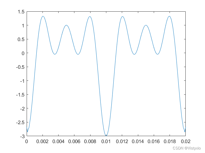
6.3 MATLAB绘制的希尔伯特变换图像